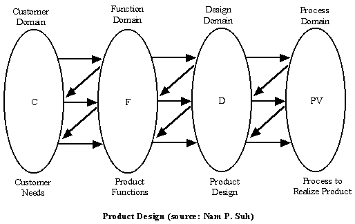
Suh’s theory of design specified that all designs could be represented in four domains:

Suh was searching for general principles, or laws, which govern good designs. The theory that followed proposed two principles, or Axioms, that could be used to describe "good designs." The first of these axioms focuses on the relationship between the functional domain and the design domain.
The thesis is as follows: The customers' wishes are often stated in non-engineering terms (e.g. A stereo system must sound good). Further, several of the requirements may be implicit, not explicitly stated. The engineering designer must identify and convert these requirements to somewhat more engineering specific requirement (e.g. the Signal to Noise ratio of the stereo must exceed 100 decibel) Thus, the customers' needs are converted into a set of functional requirements that will eventually be satisfied by the design. The actual design artifacts that satisfy each of the functional requirements lie in the design domain (e.g. a particular combination of pre-amplifier and power amplifier that yield the required signal amplification).
As an aside, one can see why techniques such as Quality Function Deployment (QFD) can be employed in the mapping from the Customer domain to the Functional domain. QFD is good way to identify which of the customers' requirements are more important and must manifest themselves in the form of an entry in the functional domain, and which may be ignored to satisfy other constraints such as cost, time to market etc.
Thus, each functional requirement must be linked to at least one of the design parameters, and each design parameter must exist to satisfy (to be more accurate, to affect) one or more of the functional requirements.
Axiom #1. The Independence Axiom. A good design is made up of design parameters that result in the independence of the functional requirements from each other.
Suppose a design has n design parameters. A small change in any design parameter may cause some deviation from the ideal value of the j-th functioanl requirement. Then one could write:

Where FR's are the functional requirements, and DP refers to the design parameters.
Of course, if a design parameter has no effect on a particular FR, the corresponding term inside square brackets will be zero.
The first axiom qualitatively looks at the values of these partial derivative terms, distinguishing between those that are zero, and those that are finite.
A matrix representation of this relationship can be shown as follows:
|
FR1 |
X |
0 |
0 |
DP1 |
||
|
FR2 |
= |
0 |
X |
0 |
DP2 |
|
|
FR3 |
0 |
0 |
X |
DP3 |
Where the X's imply non-zero values, and FRi and DPj represent the differential values of the parameters. The form of the square matrix, sometimes called the design matrix, is used to depict good or poor designs. If it is a diagonal matrix as shown above, the design is called uncoupled, and is ideal. If the DPi's and FRi's can be shuffled around to lead to a triangular matrix, the design is called decoupled, and is acceptable. If however, the matrix cannot be converted to a triangular matrix, the design is called coupled, and suggests a poor design which needs to improved.
The logic behind these directives has been described in your handouts. I will only point out that a coupled design makes it necessary to iterate in order to implement the design parameters (Why ?).
Axiom #2: The Information Content Axiom. Minimize the information content of the design.
This axiom states that the designs most likely to succeed have the minimum information content. Of course, one can only compare the information content of rival designs which can satisfy all the required functional parameters. The intent is to describe the information content by means similar to those used in information theory of Shannon; however, this axiom has been (more or less) equivalently described in terms which are more easily computed. Following are some of the definitions, and some comments about the underlying assumptions.
Information content , I = log (1/P), where P is the probability of success.
In keeping with Shannon's theory, Suh uses Log2, but the axiom works irrespective of the base you use for the log scale, as long as you stick to the same base for each computation (Why?).
Notice that when a design is certain to succeed, P = 1, resulting in I = 0. Also, since P must lie within [0, 1], I can only be positive.
How do we compute the probability of success? We first consider a single FR, satisfied by a single DP.
Suppose that the acceptable tolerance range for a functional requirement is [LSL, USL]. We call this the design range.
Suppose that the corresponding DP is distributed normally about some mean, as shown in the figure below.
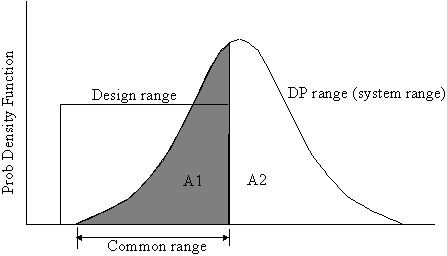
Figure 2 (source: Mats Nordlund)
Clearly, those instances of the DP which contribute to the distribution shown in the shaded area, A1, are acceptable designs (successes), whole those that fall outside this range, in the area A2, are unacceptable (failures).
Thus the probability of success, P = A1/(A1 + A2).
Of course, if the Design Parameters are distributed uniformly over the system range (uniform distribution instead of normal), then one can use the simpler formula:
Probability of success, P = common range/system range.
Yet another terminology, defines the probability of success, P = tolerance/range.
Where tolerance = common range, and range = DP range (which must be uniformly distributed).
Multiple FR's and DP's:
This case is a little more tricky. We deal with the simplest: An uncoupled design. Assume that an uncoupled design has two FR's and therefore two DP's. Independence of the FR's (because design is uncoupled) implies that the probability of success of the design, is the resultant probability of success of the DP's independently.
From high school math, we know that for independent events A and B, P(A and B) = P(A) * P(B). This leads us to the information formula, for DP1 and DP2 combined, as:
P = log 1/ (P1*P2) = log ( (1/P1 )*(1/P2) ) = log ( 1/P1) + log( 1/ P2).
That is: in an uncoupled design, the total information content equals the sum of the information content for the individual DP's.
Axiomatic Design and Mfg System Design
Sohlenius developed the structure of Mfg Sys Design within the framework of Suh's theory as follows:
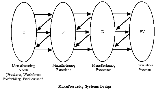
Figure 3. (source: Nam Suh)
The relation of Product design and manufacturing system design is captured very nicely in the following figure. In addition, the figure also shows how other design methodologies are applied to the different tasks.
Note how other dominant technical methods can be used within the overall framework of the Manufacturing System Design.
Quality Function Deployment is used primarily to involve the customer actively in development of the product and the product range. It provides the methods to capture the perceived importance of different features of a design are explicitly from the customer base (unlike traditional systems where this was done purely based on the experience of the designer.)
Another interesting feature is the reconciliation between the useful Taguchi methods and Axiomatic design. This relationship has been explained before in the notes. While Axiomatic design is useful in general at the conceptual design stage, Taguchi methods provide very explicit guidelines at the detailed design stage, in the determination of tolerances and the setting of the design parameters. This is show further through some of the figures 5-7.
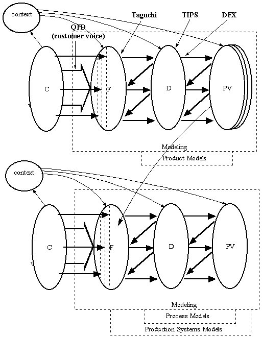
Figure 4. (source: Gunnar Sohlenius)
Taguchi methods and the Axiomatic Design Process

Figure 5. (source Gunnar Sohlenius)
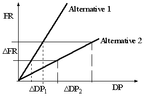
Figure 6. (source Gunnar Sohlenius)
Typically, the design tolerances are specified as tolerances of the FR's. The figure above shows that a design with lower stiffness (i.e., FR_DP curve is flatter, as in Alternative 2), will provide an easier one to achieve. This is since a larger tolerance in DP can still provide a design with the same tolerance range as the specified value in the FR.
This is easy to see in the traditional methods, in terms of the step shaped Quality Loss Function. Is it also true in case of Taguchi ?
Yes. For a given value of A0, the Taguchi loss function is flatter for a larger range of values of tolerance. Therefore, for a part which is out of tolerance by the same amount, d, will have lower loss of quality when the loss curve is flatter.
In the figure above, we assume that the variation of DP's with FR is linear over the range of acceptable designs. In general, this may not be true. If the curve is non-linear, Taguchi again provides us a strategy to select the design parameter range where the curve is flatter, if possible. Designs operating in the flatter range can provide low cost solutions with same tolerance of FR's. This is shown graphically in Figure 7.
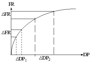
Figure 7. (source: Gunnar Sohlenius)
Prof Sohlenius also compiled a short document summarizing the basic principles in Axiomatic Design. Here is a link to this document.
Notes based on the teaching material for IEEM 513 Manufacturing Systems
Design, spring 1998, of Prof Gunnar Sohlenius. References for the materials
covered include papers of Mats Nordlund and Gunnar Sohlenius, and the
following texts:
The Principles of Design, Nam P Suh, Oxford University Press.