Johnson's Algorithm For Scheduling
In the notes below, I shall try to present some intuition about Johnson's algorithm, and why it works for scheduling of manufacturing systems. At the end of it all, we shall see what kind of systems it can be usefully applied to.
One Machine, Two Jobs
We begin the discussion with the simplest scheduling problem: You go to Park 'n Shop to buy a can of Coke. At the check-out counter, just before you, is a lady with a large basket of groceries. The lady allows you to go ahead of her, pay for your coke in 1/2 min, and then presents her basket to the clerk who takes 5 min to check and bag her order.
This lady was using a well known rule for scheduling single processor systems: Scheduling shortest job first will result in minimum average (and total) waiting time.
In the example above, if the system worked as First-Come, First-Served, then the total waiting time would be = 0 min for the lady + 5 min for you = 5 min.
If you go first, then the total waiting time = 0 min for you + 1/2 min for her = 1/2 min !
One machine, N Jobs
In fact, this logic easily extends to the case for 1 Machine (or server), and N Jobs. By scheduling the jobs in the sequence of shortest time ... longest time, you are guaranteed to get the minimum waiting time (total, or average).
Proving this is quite simple: try it ! [Hint: You can use mathematical induction.]
Notes:
While the above example is simple, it can give a few lessons. An important lesson is: Know your objectives !
For instance, if your aim is to minimize the makespan (which is defined as the time between the moment you start the first Job, till the time you end the last Job), then it does not matter how you schedule a single server system ! However, if your objective is to minimize average waiting time, then the Shortest Job first rule is optimum (this rule is called the SPT rule, or the Shortest Processing Time rule).
Two Machine Cases:
The mathematics is much more difficult as soon as we start to schedule two machine systems. We start with the following system:
There are three parts, P1, P2, and P3. Each needs to be processed first on Machine M1, then on Machine M2. The processing times are as follows:
|
Parts |
|||
|
Machines |
P1 |
P2 |
P3 |
|
M1 |
6 |
2 |
8 |
|
M2 |
4 |
4 |
4 |
We could have 6 possible sequences for the parts: 1-2-3, 1-3-2, 2-1-3, 2-3-1, 3-1-2, and 3-2-1.
For any sequence, Machine 1 will start working at T=0, and work till T= 6+2+8 = 16.
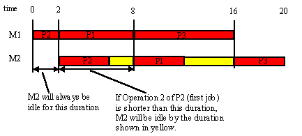
Notice, however, the utilization of M2:
Of course, in the above example, I deliberately chose all 2nd operations of equal length, to make it easy to identify the optimal sequence [Which one is it ?] [Hint: it uses SPT for Machine 1].
Now let’s look at this more carefully, using Gantt charts.
Note: whatever sequence we use, it is clear that Machine 1 will begin at T=0, and be fully utilized for the duration = sum of Operation 1 durations for all parts.
This is ALWAYS true !
Therefore, all scheduling of Parts we perform must concentrate on trying to make the Gantt chart for Machine 2 as compact as possible.
Case 1. A Simple example

Clearly, we cannot do much better than this (since Machine 1 must operate till T=16, and thereafter, Machine 2 still needs 4 units of time to complete the last job on Machine 1.)
Some more observations:
It appears to make sense to ALWAYS put the shortest job of Machine 1 at the beginning, for this will minimize the initial idle time of M2.
Also, since Machine 2 must work on the second operation of the final job after all work on Machine 1 is finished, it also makes sense to ALWAYS put the shortest operation of the second Machine at the end of the schedule.
What can we say about the jobs in between ?
Mainly, we would like to minimize the yellow portions as much as we can. How can we do this ? Johnson noticed that this can be done if
Now we have gained enough intuition to develop one form of Johnson's algorithm. We shall first try another example, and then write the algorithm.
|
Parts |
|||
|
Machines |
P1 |
P2 |
P3 |
|
M1 |
30 |
14 |
30 |
|
M2 |
25 |
28 |
19 |
Using our logic above, the shortest operation on Machine 1 is P2, so we schedule it first (luckily, the operation 2 for P2 is the longest, so that is also in accordance with Johnson's 2nd observation above). Also, the shortest operation on Machine 2 is P3, so we schedule it last. Hence we get the sequence: P2-P1-P3.
Is this the best sequence ? Try out the different Gantt charts to convince yourself.
Once you are comfortable with this, you can understand the logic behind Johnson's algortihm, which I state below:
Two Machines, N Parts:
Part Pi has two operations, of duration Pi1, Pi2, to be done on Machine M1, M2 in that sequence.
Step 1. List A = { 1, 2, …, N }, List L1 = {}, List L2 = {}.
Step 2. From all available operation durations, pick the minimum.
If the minimum belongs to Pk1,
Remove K from list A; Add K to end of List L1.
If minimum belongs to Pk2,
Remove K from list A; Add K to beginning of List L2.
Step 3. Repeat Step 2 until List A is empty.
Step 4. Join List L1, List L2. This is the optimum sequence.
Let’s see this with the help of another example:
|
Parts |
||||||
|
Machine |
P1 |
P2 |
P3 |
P4 |
P5 |
P6 |
|
M1 |
6 |
10 |
4 |
7 |
6 |
5 |
|
M2 |
4 |
8 |
9 |
2 |
3 |
6 |
Step 1.
A = { 1, 2, 3, 4, 5, 6}
L1 = {}
L2 = {}
Step 2.1.
Shortest job is P42; Remove Part 4 from list A, and add Part 4 to beginning of list L2
A = { 1, 2, 3, 5, 6}, L1 = {}, L2 = { 4}
Step 2.2.
Of remaining parts, shortest operation is P52, Remove Part 5 from A; Add Part 5 to beginning of List L2.
A = { 1, 2, 3, 6}; L1 = {}, L2 = { 5, 4}.
Step 2.3.
Now, there are two shortest remaining operations: P12, P31.
Since they are on different machines, we can randomly pick either;
If both choices are on machine 1, pick the one with the longer operation 2 first;[Why ?]
If both are on machine 2, pick the one with the longer operation 1 first. [Why ?]
We select (randomly) Part 1. Remove Part 3 from list A, add Part 3 to end of List L1.
A = { 1, 2, 6}, L1 = { 3}, L2 = { 5, 4}
Step 2.4.
Shortest remaining operation is P12, so we remove Part 1 from List A, and add it to beginning of List L2.
A = { 2, 6}, L1 = { 3}, L2 = { 1, 5, 4}
Step 2.5.
Shortest remaining operation is P61; Remove Part 6 from A, add to end of List L1.
A = { 2}, L1 = { 3, 6}, L2 = { 1, 5, 4}
Step 2.6.
Shortest remaining operation is P22. Remove Part 2 from A, add to beginning of L2.
A = {}, L1 = { 3, 6}, L2 = { 2, 1, 5, 4}
Step 3. List A is exhausted. Join L1 and L2, to get the optimum sequence:
{ 3, 6, 2, 1, 5, 4}.
Convince yourself that this is the best sequence.
Johnson's algorithm and Multiple Machines
Johnson's method only works optimally for two machines. However, since it is optimal, and easy to compute, some researchers have tried to adopt it for M machines, (M > 2.)
The idea is as follows: Imagine that each job requires m operations in sequence, on M1, M2 … Mm. We combine the first m/2 machines into an (imaginary) Machining center, MC1, and the remaining Machines into a Machining Center MC2. Then the total processing time for a Part P on MC1 = sum( operation times on first m/2 machines), and
Processing time for Part P on MC2 = sum( operation times on last m/2 machines).
By doing so, we have reduced the m-Machine problem into a Two Machining center scheduling problem. We solve this using Johnson's method, and based on the sequence obtained, schedule jobs on the m-individual machines using the usual Gantt chart method.
Of course, since our choice to combine the first m/2 machines into a machining center is purely arbitrary, it is totally acceptable to break (partition) the list { 1, 2, …, M} at any point to generate our imaginary Machining Centers. Some researchers have suggested a method that involves trying several different alternatives, tests the sequence resulting from each option through Gantt charts, and picks the best option from among these choices.
A final Note
You may have noticed that Johnson's method only works when each part has the SAME set of machines to visit, in the SAME sequence. Clearly, this is an important restriction. In practical conditions, Johnson's method is most useful in scheduling operations for a family of parts within a group (since most parts of a family require similar processing) -- and hence its use in Group Technology.