The allocation of a set of well defined resources to a set of well defined tasks subject to some well defined constraints, in order to satisfy a specific objective.

Applications:

General Applications:

• computer systems
• hospital administration
• transportation management
• manufacturing and production
• classroom allocation, examination planning etc.

Manufacturing Applications

• Textile manufacturing
• Semiconductor manufacturing
• Process industry
• Product assembly

Note that all production of parts takes place in batches, and the batch size can vary from 1 (in job shops) to a million parts (in an assembly line).

Depending on how the jobs move around in the shop floor (that is, the sequence in which they visit machines, or processors) we can classify manufacturing systems as one of:

Serial systems (also called flow shops) [examples: assembly lines, transfer lines] or

Non-serial systems [examples include FMS, job shops].

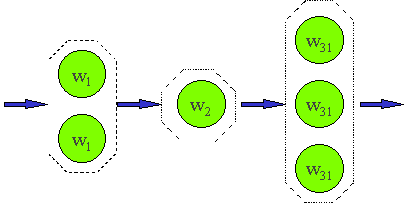
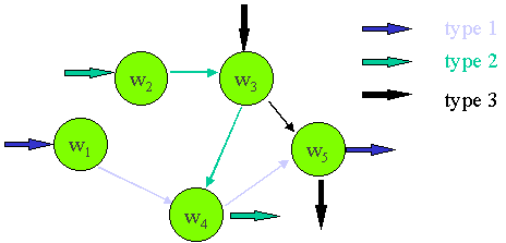
The following figures summarize some typical scheduling/flow types.

Figure 1. assembly line/flow shop

Figure 2. Assembly lines/flow shops with multiple routes and buffers

Figure 3. Flexible flow shop

Figure 4. Job shop

In order to formulate a scheduling problem, people use some form of math optimization method (either an LP, or more commonly, an NLP, solved using DP).

Terminology:

• N: number of jobs
• M: number of machines
• d_i: due date for job-i
• Pij: processing time for job-i on machine j. We also need to specify setup time.
• r_i: release date of job i
• w_i weight of job-i: i.e. its importance relative to other jobs.

Solution dependent measures:

• C_i: completion time of job-i
• F_i: length of time the job is in the system (flow time).
• L_i: lateness of the job-i ( C_i - d_i)
• T_i: tardiness of the the job-i ( max( 0, L_i) )

Typical specification of scheduling problems involves first specifying the problem in the format:

N/M/A/B

N: 1, 2, or N (number of jobs)

M: 1, 2, or M (number of machines)

A: the job flow pattern (discussed later in these notes), and

B: the performance measure (e.g. average flow time)

NOTE: The performance measure is always stated in terms of a measure that needs to be MINIMIZED, so the B-field only shows the criterion, not the optimization condition.

Usually, we are interested in N-jobs problems, and therefore we may specify only the last three of these in the problem, that is, M/A/B specification. Some people call this the a/b/g specification)

Notations:

	
a	machine environment
	
b	processing characteristics/constraints 
	
g	objective functions

a-field notations:

1	Single machine
Pm	m identical machines in parallel; job-j can be processed by any one of them.
Qm	m machines in parallel with different processing time; job-j can go to any one.
Rm	m unrelated machines in parallel; each job can go to a particular one (or one of a subset) of these m.
Fm	Flow shop: m machines in series. Each job goes to each machine. All jobs have same routing. Most common schedule is a permutation schedule (FIFO at each machine)
FFs	Flexible flow shop. s-stages in series, each stage has 1, 2, or more machines, and each job may be assigned to exactly one machine in each stage.
Om	Open shops. Each job must visit each of m machines; each job has unique route; If jobs can visit same machine more than once, then Om|recrc|
Jm	m machine job shop. Each job can visit one or more machine, and has its own route.

b-field notations:

NOTE: while any given problem specification will contain only one entry in the a-field, it may contain several comma-separated values in the b-field.

g-field notations:

	Cj :	Completion time

	Lj :	Lateness (Cj - dj)

	Tj :	Tardiness, ( = max{ 0, Lj} ).

	Uj :	Unit penalty ( = 1, if Tj is non-zero, 0 otherwise).)

	Cmax :	Makespan ( = completion time of the last task of the last job to be completed)

	Lmax :	Maximum lateness.

	= total weighted completion time. Weight of each job indicates its relative importance.

	= total weighted tardiness.

	= total weighted unit penalty.

	= total weighted discounted completion time.

Each of the above are objectives that must be minimized. Typically, a shop manager will select his/her favorite from among these objectives to schedule their factory. Most of these are self explanatory, except for the last one. There, we see use, instead of a linear importance of the completion time, a non-linear function, which (depending upon the rate, r, makes jobs with closer completion times relatively more important that others.)

Having specified the problem, we still need to (a) formulate the problem, and then, (b) solve the problem.

It turns out that it is neither easy to formulate, nor to "solve" any useful sized problem. We demonstrate this complexity by the simplest of examples:

Consider a Flow shop, with the following jobs:

There are 4 machines, and 4 jobs. Assume that setup times are included in the processing times.

The solution is made simpler since it a is a flow shop: each job must visit the machines in the same sequence (1-2-3-4).

How many solutions can this system have ? (how many possible solutions need we consider to select the best one ?)

Note: in general, the worst case would make us consider the order of n!^m schedule possibilities.

Clearly, a difficult problem. so let's simplify the problem a little bit: Assume that the jobs must be processed on each station is the sequence in which they arrive. [this is called a permutation schedule]. Now, how many solutions need one explore ?

Ans.: Still of the order of n! (in the above case, 4! = 24 schedules.)

Factorial-n is a large number, for a typical factory manager, who may be scheduling between 40 and 100 job orders in any given week of production. In fact, try solving the above problem, and you will find that even for the case of 4-jobs, 4-machines, it takes you an afternoon to discover the best schedule. And all this, assuming that all jobs are ready at t=0.

The outcome of all this is that solving scheduling problems is tough. We therefore resort to the following:

1. We use a computer to perform a lot of the calculations. This requires development of complex computer programs.
2. We use some simple scheduling rules, by which we can get "a solution", not the best solution.

Several well known scheduling heuristics have been employed by different people, and several have been found to yield 'good' solutions. Besides, many such heuristics make some kind of manufacturing sense, and are therefore easily adopted by practitioners. Common among these are EDD (earliest due date: among all remaining jobs, schedule the one with the earliest due date first), FCFS (first-come, first-scheduled), SPT (shortest processing time: schedule the job with the shortest processing time first), the COVERT rule (schedule the job with the minimum C/T, where C is the time remaining till the expected Completion time for a job, and T is the processing time for the job; the name of the rule emerges from reading its formula: C-over-T), SS (shortest slack time first: slack is the duration between the job arrival time and its expected due date), etc.

Another heuristic method of scheduling, useful in flow shops, was analyzed in some more detail when we studied Cell scheduling and GT: Johnson's algorithm.

One of the powerful tools in the formation, display, and manipulation of schedules is the familiar Gantt chart.

In the lab, we shall try out the Lekin scheduling software. This software was developed by Pinedo et al. You are free to borrow copies of the educational version of this software ( or download them).

Lekin scheduling software is copyright protected, from Stern School of Business, New York University. Information through Prof Michael Pinedo: mpinedo@stern.nyu.edu).