Search is useful to find optimal (or, at least, good) solutions to discrete problems. Most discrete problems will be modeled in terms of a set of variables that can take only discrete values (e.g. variables can only be 0 or 1, or they can only be integers). The optimum solution maximizes (or minimizes) the value of a function (called the objective function) of these variables. The values of the variables that optimize the objective function make up the optimal solution.
Such problems are very common in everyday life -- in engineering, or outside engineering.
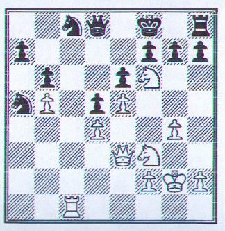
Example 1. The decision about which is the best move at any point in a chess game is a discrete problem (figure 1).
Figure 1. Kasparov vs. Kaiumov, Tbilisi 1976
In the above figure, White (to move) has 34 possible moves (R=14, Nf6=7, Nf3=5, Pg4=1, Ph2=2, K=5). For each move, Black will have a finite number of options for response; and so on.
Example 2. The eight-queens problem
The objective of this popular puzzle: place 8 queens on an empty chess-board such that no queen will attack any other. It is obvious that no more than 8 can be so placed, since if there are 9, at least two must be on the same row, and will therefore attack each other.
Solving this puzzle manually is not too easy; but it is easy to set up a computer program that will determine a solution quite quickly by exhaustive searching. A simple search logic would place the 8 queens sequentially:
The first queen can be placed on one of 64 squares;
The 2nd queen can thereafter be placed on any of the remaining 63 that are not attacked by the first; … and so on till the 8th queen is successfully placed.
Note: one can, of course be smarter and observe the following: each row must contain exactly one queen; so we may just assign the first queen row 1, the second, row 2, and so on. Thus the search can be reduced greatly. Figure 2 shows a typical stage of this search.
Figure 2. A search space for the 8-queens problem after three queens are placed
Modeling the Search Space: Graphs
In most examples for searching, a common model is a graph. A graph is a structure of two sets: a set of nodes, and a set of edges, each connecting two nodes. For each search, you must first decide what the meaning of each node is. In the first example, one choice is to represent each node by the move made in a step (represented by which piece is moved, from which square, and to which square). Another choice could be to represent the entire board after a move is made (that is, the location of each piece).
In this case, the first choice appears better, since it requires much less information to be stored for each node (which means less memory requirements for the program). But of course, a program evaluating the state of the board after any move must know the positions of each piece on the board -- thus, along with each node, one must also store all the moves made before it (in graph terms, the path from the start node to the current node). But let's leave these details till later, and assume that the state of affairs on the board can be efficiently computed corresponding to any node.
For a chess program, we may introduce a dummy start node, representing the opening position. From there, each legal move by White will represent a node. For any node, there will a set of edges, each one connecting the node to a feasible response by Black; and so on.
Notations:
In the context of searching, the following convention is useful: Each node shall represent a sub-problem (more precisely, we may say that each node is an encoding of a sub-problem.) For each graph, we shall assign a special node, called START, which represents the initial problem. Some pairs of nodes are connected by an edge (directed edges are called arcs) – edges represent the operators available to the problem solver (e.g. in Chess, each arc represents a legal move leading from the parent node to the child node. The number of edges going out of a node is the degree of the node.
A graph in which each node has at most one parent is a tree.
In some graphs, each edge has a weight associated with it. You may travel from one node to another only along edges; when traveling between node A and node B, the total weight collected is the sum of weights of edges along which you traveled in moving from A to B.
Note that in many search problems, it is not feasible, nor wise, to generate the entire graph at the outset – it may be too large! Thus, searching the graph requires two basic steps: the ability to evaluate a given node (at least enabling us to discern if it represents a problem that is solved trivially, or is a goal node), and to expand a given node. Node expansion is the generation of all the successors of a given parent node.
Sometimes, we may need to distinguish between node expansion and node generation. In node generation, the successors of a parent node are only created one-at-a-time. This distinction is mostly useful from a programming point of view, and does not affect the search procedure in any way. It leads to a better implementation of depth first searching, called backtracking.
Exhaustive searching
Depth first (LIFO)
Depth first searches are implemented using a data structure called stack, which is basically a list, maintained as follows. You can place or remove members from the list at any time. If you insert a member into a stack, it is placed at the beginning. If you remove a member from the stack, the first member is removed. This is the same as a Last-In-First-Out policy (LIFO)
This is a simple strategy to implement. The only things we must be careful about are:
If the graph is very large (or infinite), the search may just keep continuing searching deeper and deeper along some fruitless path. Hence, we must provide a mechanism to recover from disappointments, that allows us to back up, and begin searching along a new path. Thus, we shall provide a user-defined MAX-DEPTH, which will trigger a search path to CLOSE once we have searched to this depth without reaching the goal.
Depth-first Search Algorithm
INPUTS: search graph G, depth bound MAX-DEPTH, start node S, goal GOAL.
// We shall use two lists, OPEN and CLOSED to keep track of nodes.
NOTES:
Figure 3 shows the depth-first search tree for a 4-queens problem. Circled nodes are CLOSED, and nodes in a triangle are dead-ends. The successor function generates, in the i-th level, the board positions available for locating the queen in the i-th row.
Figure 3. Depth-First Search for the 4-Queens Problem
Breadth first (FIFO)
Depth first operates based on a LIFO strategy for handling successors. If instead, we use a FIFO (First-In-First-Out) policy, then the characteristics of the search are quite different. In this case, all nodes at a lower depth level get priority. Hence, all nodes at a given depth are first explored, before exploring the nodes at the next higher depth.
Breadth First Algorithm
This algorithm is exactly the same as the one for Depth first, except the last stage of Step 6, which will now read:
insert Snj at the end of OPEN;
Notice that by putting the newly expanded nodes at the end of the list of nodes to be explored, we give a higher priority to the nodes generated earlier -- hence this is a FIFO policy. Using the 4-queens problem again, the following is the breadth-first search tree.
Figure 4. Breadth-First Search Tree for the 4-Queens Problem
Best First
Both depth- and breadth-first search policies are sometimes called uninformed policies, since they systematically and exhaustively look for solutions along every path, treating each path as if it is equally likely to lead to the goal. Sometimes, heuristic functions may allow us to identify some paths as more promising than others. Such strategies may reach the goal faster than uninformed searching.
We are still searching over a graph. At any stage, the decision we need to make is: which node of OPEN should be expanded. For simplicity, let us assume that each node represents a partial solution to our problem – of course, it may or may not be part of a valid, complete solution. Assume we can define a function, f( n) à R (n is the node, and R is the set of reals), which gives a numerical measure of the potential of n to lead to the goal. The best first policy uses such functions to decide the next node of OPEN that must be expanded.
There are several variations of the best first strategy. We shall only look at a specific variant, in an application of our interest: scheduling N jobs on 1 machine.
Recall that we could minimize the total waiting time in scheduling N jobs that are all released at t= 0 by using SPT. Now we consider the case where the different due dates, and a lateness penalty is charged for each job that is late. The objective is to minimize the total cost. In this case, one must search for the best (for a given objective) among N! permutations. One way to solve this problem is with a variation of the best first, called a Branch-and-Bound search.
Some notations for the Scheduling Problem:
Pi = Process time for the i-th task
Di = Due date for the i-th task
Li = Cost charged per unit time of tardiness for task i. If task I is completed t units of time after its due date, we incur a cost of (Li X t).
The objective is to minimize the total tardiness cost.
In setting up the branch and bound search, one has to select the heuristic function carefully. In this case, it is convenient to set up a function that yields a bound on the cost if we set up a backward-planning search. That is, the first level of nodes from START indicate possible choices of the last task we shall do. This gives us a means to compute a lower bound on the total tardiness cost. The algorithm is as follows:
Branch-and-Bound for N-jobs 1-Machine Scheduling:
OPEN = {}
The algorithm above can be demonstrated with the help of a simple example.
Data:
| Job | Pi | Di | Li |
| 1 | 37 | 49 | 1 |
| 2 | 27 | 36 | 5 |
| 3 | 1 | 1 | 1 |
| 4 | 28 | 37 | 5 |
Figure 5 shows the branch and bound search tree for this data.
Figure 5. Branch and bound search tree
Non-optimal (heuristics) Commonly used in Scheduling Problems:
While best first techniques may prune the search tree somewhat, their worst-case performance is no better than combinatorial. For several problems, they may require prohibitively large computation times. Hence several scheduling systems use some common heuristics that are known to yield reasonable/acceptable solutions (or at least, good starting solutions which may be used as a basis for the selected solution.) The most popular among these include the following.
EDD (Earliest Due Date):
This policy arranges the tasks to be started in the sequence of ascending due dates. Therefore, it provides a schedule in O(nlogn) time.
SPT (Shortest Processing Time)
Schedule tasks in order of ascending processing times for the tasks. We studied this heuristic when we looked at Johnson's algorithm for cell scheduling.
COVERT (Cost OVER Time rule)
The COVERT rule works as follows.
TT = sum of all processing times
RT = Sum of processing times of al tasks still remaining to be scheduled
ST = Starting time for the next scheduled task; 0 for first task
CF = Coefficient calculated as below
PRi = Priority of task i (see below)
COVERT Algorithm:
Exercise:
Apply the above heuristics to the data used for the branch-and-bound search, and compare the results with the optimum (corresponding to the objective of minimization of the lateness cost).
Sources:
Pearl, J., Heuristics, Addison Wesley 1984
Sule, D. R., Industrial Scheduling, PWS Publishing, Boston, 1997