We have studied the ER diagram as a tool to describe the conceptual model of the Universe of Discourse.

In this lecture, we show a formal method to convert this conceptual model into a logical model called the Relational Model.

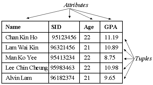
We shall represent a relation as a table of values. Each column of the table has a title or header, called an attribute. Each row is called a tuple.

• Domain: a set of atomic values that an attribute can take

• Attribute: a name to suggest the meaning of a particular domain. Each attribute A_i has a domain, dom(A_i).

• Relational Schema: a relation name, R, and a set of attributes, A_i, that define the relation.

• Degree of a Relation: the number of attributes in the relation's schema.

• Tuple, t, of R( A1, A2, A3, …, An): an ORDERED set of values, < v1, v2, v3, …, vn>, where each v_i is a value from dom( A_i).

• Relation Instance, r( R): a set of tuples.

Example of a relation:

1. The tuples in a relation are not considered to be ordered. In other words, a table like the one above, with the rows appearing in a different sequence is considered to be logically identical.

 

2. Once the schema, R( A1, A2, A3, …, An) is defined, the values, v_i, in each tuple, t, must be ordered as t = <v1, v2, v3, …, vn>

 

3. Values in a tuple: each value in a tuple is considered ATOMIC

Each relational schema must satisfy the following four types of constraints.

1. Domain constraints

Each attribute A must be an atomic value from dom( A) for that attribute.

Examples of domains could be: integer, real numbers, character, fixed length string, date etc.

 

2. Key Constraints

Superkey of R: A set of attributes, SK, of R such that no two tuples in any valid relational instance, r( R), will have the same value for SK.

 

Therefore, for any two distinct tuples, t1 and t2 in r( R), t1[ SK] != t2[SK].

 

Key of R: A minimal superkey. That is, a superkey, K, of R such that the removal of ANY attribute from K will result in a set of attributes that are not a superkey.

 

EXAMPLE

 

CAR( State, LicensePlateNo, VehicleID, Model, Year, Manufacturer)

is a relational schema, with two keys:

 

K1 = { State, LicensePlateNo}

K2 = { VehicleID }

Both K1 and K2 are superkeys.

 

K3 = { VehicleID, Manufacturer} is a superkey, but not a key (Why?).

 

If a relation has more than one candidate keys, we can select any one (arbitrarily) to be the primary key. Primary Key attributes are underlined in the schema:

CAR( State, LicensePlateNo, VehicleID, Model, Year, Manufacturer)

 

3. Entity Integrity Constraints

A database normally contains many relational schemas, R1, R2, …, Rn. the set of all relational schemas belonging to the database is called a relational database schema, S.

 

S = { R1, R2, …, Rn}

 

Entity Integrity: The primary key attribute, PK, of each relational schema R in S cannot have null values in any tuple. This is because PK is used to identify the individual tuples.

 

Thus, t[PK] != NULL for any tuple in r( R).

 

4. Referential Integrity Constraints

Consider a referencing relation, R1, and a referenced relation, R2. Tuples in the referencing relation, R1, have attributed FK (called foreign key attributes) that reference the primary key attributes of the referenced relation, R2. A tuple, t1, in R1 is said to reference a tuple, t2, in R2 if t1[FK] = t2[PK].

A referential integrity constraint can be displayed in a relational database schema as a directed arc from the referencing (foreign) key to the referenced (primary) key. Examples are shown in the figure below:

Now we are ready to lay down some informal methods to help us create the Relational schemas from our ER models. These will be described in the following steps:

1. For each regular entity, E, in the ER model, create a relation R that includes all the simple attributes of E. Select the primary key for E, and mark it.

 

2. For each weak entity type, W, in the ER model, with the Owner entity type, E, create a relation R with all attributes of W as attributes of W, plus the primary key of E. [Note: if there are identical tuples in W which share the same owner tuple, then we need to create an additional index attribute in W.]

 

3. For each binary relation type, R, in the ER model, identify the participating entity types, S and T.

 

• For 1:1 relationship between S and T

Choose one relation, say S. Include the primary key of T as a foreign key of S.

 

• For 1:N relationship between S and T

Let S be the entity on the N side of the relationship. Include the primary key of T as a foreign key in S.

 

• For M: N relation between S and T

Create a new relation, P, to represent R. Include the primary keys of both, S and T as foreign keys of P.

 

4. For each multi-valued attribute A, create a new relation, R, that includes all attributes corresponding to A, plus the primary key attribute, K, of the relation that represents the entity type/relationship type that has A as an attribute.

 

5. For each n-ary relationship type, n > 2, create a new relation S. Include as foreign key attributes in S the primary keys of the relations representing each of the participating entity types. Also include any simple attributes of the n-ary relationship type as attributes of S.

We have seen the informal procedure to map the ER model into a logical model (relational database schema). How do we know that this is a good schema?

We shall now study the formal theory which can help us to understand (a) what is a good relational database design, (b) why it is good, and (c) how do we design good relational database schemas.

To do so, we shall learn the concepts of Functional dependencies and Normal forms.

We shall use this database for our examples.

To give us some motivation, let us first see what kinds of problems can arise if we fail to design the database properly.

1. Redundant Information in Tuples and Update Anomalies

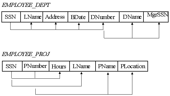
Consider a (poorly) designed database where the Employee and Department information is planned in one table, and the Employee and Project information in another table:

 



 

Problems:

 

( a) Information is stored redundantly -- repeated information => wasted storage.

For example, if 5 employees work for Department number 4, then the department name and manager's SSN for Department 4 is stored 5 times in the table.

 

( b) Insertion anomalies. When we enter the record for a new employee, we must specify ALL data fields for his department correctly. For example, if a new employee joins Dept 5, then we must ensure that the data entered for Dept 5 in the new record is consistent with the data for Dept 5 in all earlier records of other employees of Dept 5.

 

( c) Deletion Anomalies. If a dept has one employee working in it, and we delete the information of this employee, then the information of the department is also lost. We may not want this to happen.

 

( d) Modification Anomalies. If we modify a value, we must make the entire table consistent very carefully. For example, if an employee changes departments from Dept 5 to Dept 4, then his entire record must be changed, not just his DNumber field. If a department changes its manager, the entire table must be scanned and modified.

 

2. Null values in Tuples

In general, we should design tables which have the fewest NULL value entries. If an attribute has NULL value very frequently in a table, it should be placed in a separate table (along with the primary key).

 

3. Spurious (false) Tuples

One way to alleviate several of these problems is to ensure that our relational database schema is normalized. We shall now study normalization.

Functional dependencies (FDs) are used to specify formal measures of the "goodness" of relational designs.

FDs and Keys are used to define normal forms for relations. FDs are constraints that are derived from the semantics of the universe of discourse (that is, the meaning and inter-relations of the data)

A set of attributes functionally determines a set of attributes Y

if the value of X determines a unique value for Y.

This is written as: X -> Y.

The implication of the statement X -> Y is that, for any two tuples, t1 and t2,

if t1[ X] = t2[ X], then t1[ Y] = t2[ Y].

Inference Rules for FD's

Given a set of FDs, we can infer other FDs that will also be true. The rules that are used in this inference are summarized below:

A1. (Reflexive).

A2. (Augmentation).

(notation; XZ denotes X U Z, the set union of X and Z).

A3. (Transitive).

A1, A2, and A3 form a complete set of inference rules for FDs. Using these, we can also prove some additional useful inference rules:

A4. (Decomposition).

A5. (Union).

A6. (Pseudotransitive).

Closure of a set, F, of FDs, denoted F⁺, is the set of all FDs that can be inferred from F.

Closure of a set of attributes, X, with respect to F is the set X⁺ of all attributes that are functionally determined by X.

X⁺ can be calculated by repeatedly applying A1, A2 and A3 using FDs in F.

Equivalence of sets of FDs: Two sets of FDs, F and G are said to be equivalent if every FD in F can be inferred from G, AND every FD in g can be inferred from F.

Therefore, F and G are equivalent if F⁺ = G⁺.

Minimal set of FDs: A set of FDs is minimal if it satisfies the following conditions.

( a) Every dependency in F has a single attribute for its RHS (right hand side).

( b) We cannot remove any dependency from F, and have a set of dependencies equivalent to F.

( c) We cannot replace any dependency, X -> A, in F with a dependency, Y -> A, where Y is a proper subset of X, and still have a set of dependencies equivalent to F.

In general, we know the following to be true:

Disallow any composite attributes, multi-valued attributes, and nested relations.

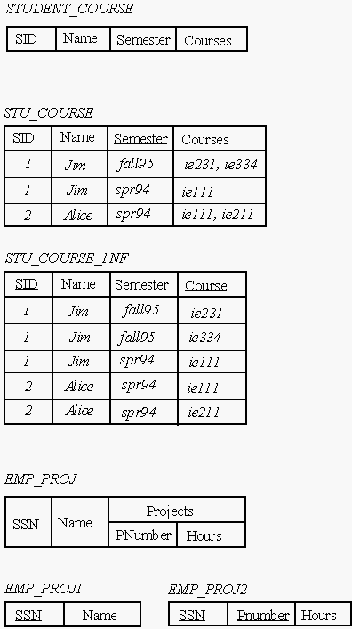
The application of the 1NF is shown in the two examples below. In the first case, The relational schema STUDENT_COURSE has a multi-valued attribute, Courses. A key for STUDENT_COURSE is {SID, Semester}. To get this schema to 1NF, we may convert the multi-valued attribute into a simple attribute, as shown in the schema STU_COURSE. What is a key for STU_COURSE ? Why ?.

In the second example, the Project information corresponding to each SSN (that is, each Employee), is a composite attribute. In this case, the Projects information corresponding to each SSN is multi-valued. Each employee may work for many projects. Therefore, to get this schema into 1NF, we must break it up into two schemas, EMP_PROJ1 and EMP_PROJ2 as shown.

Note: If the composite attribute is single-valued, then we may just use the components of the attribute in the same schema. For example, EMPLOYEE( SSN, NAME(FName, MInit, LName) ), where NAME is a single valued composite attribute, may be written in 1NF as: EMPLOYEE( SSN, FName, MInit, LName).]

2NF uses the concepts of FDs and the primary key.

Prime Attribute: An attribute that is a member of the primary key.

Full functional Dependency: A FD, Y -> Z, where the removal of ANY attribute from Y means that the FD will not hold true any more.

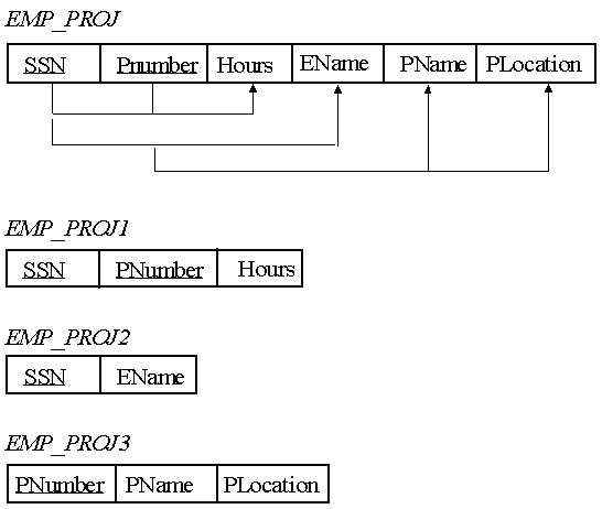
{SSN, PNumber} -> Hours is a Full FD, since neither {SSN} -> Hours, nor {PNumber} -> Hours is true.

{SSN, PNumber} -> EName is NOT a Full FD, since {SSN} -> EName is also true.

Second Normal Form: A relational schema, R, is in 2NF if every non-prime attribute A in R is fully functionally dependent on the primary key.

Transitive Functional Dependency: A FD Y -> Z that can be derived from two FDs Y -> X and X -> Z.

Third Normal Form: a relational schema is in 3NF if it is in 2NF, and no non-prime attribute A in R is transitively dependent on the primary key.

Below is an example of a schema that is not in 3NF, and how to decompose it into a pair of 3NF relational schemas.

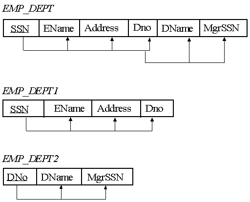
For most applications, achieving 3NF as defined above will provide an acceptable logical design. However, note that the entire process above is dependent on the (arbitrary) selection of primary keys from all possible candidate keys. There is a broader definition of 3NF which considers the existence of multiple candidate keys.

The general 1NF definition is identical to the one before.

A relational schema is in 2NF if it is in 1NF, and if every non-prime attribute A in R is fully functionally dependent on every key of R.

The general 3NF definition requires our earlier definition of superkeys ( a superkey of R is a set of attributes which contain a key of R).

A relational schema R is in 3NF if whenever a FD X -> A holds in R, then

Consider a simplified database for Government records on land sales in different districts.

Each lot of land has a unique ID number for the territory. Within each district, each lot is also assigned a lot#, which is unique in the district.

Further, the tax rate to be paid is determined by the district.

Finally, the government controls the cost of land to be uniform across the territory, so that the price can be determined by the area of the lot.

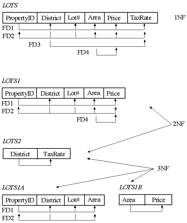
Notice: there are two candidate keys: { PropertyID} and { District, Lot#}.

TaxRate is partially dependent upon the candidate key { District, Lot#}, due to FD3.

Hence we break this schema into two parts to achieve 2NF, as shown.

LOTS2 is already in 3NF according to the general definition. However, LOTS1 violates the general definition of 3NF, since by FD4, Area -> Price. However, (a) Area is not a superkey of LOTS2; AND, (b) Price is not a prime attribute of LOTS2.

Therefore we further break LOTS1 into LOTS1A and LOTS1B to achieve 3NF.