When computers became popular, a natural result was their use in making and storing engineering drawings. Around 1970, several researchers started exploring how to solve complexproblems using the computer . By storing engineering drawings, it was still difficult for this data to be used in a program that could, for example, compute the volume (and therefore the weight) of a designed part. And what if a different section view of a part would be needed than the one in the drawing ? Baumgart, A student in Stanford university was studying the planning of robot motions in industry. To do such planning, the computer needed to decide whether some obstacle in the work-region of the robot would restrict the motion of the robot along some trajectory (this problem is called obstacle avoidance, since the planned path of the robot must avoid any collisions with obstacles). To detect collision, 3D models of the robot and the obstacles were required - because only such models can be used to check if two components will have some intersection in space. Baumgart's solution was to store enough geometric information about a solid body that could allow computing its solid properties (e.g. volume, or the determination whether a given point is inside the solid or outside); further, his data-structure also assisted in doing such computations very efficiently - which is why almost all solid modelers today are still based on his data structure. This lecture will cover that and other methods that form the basis of modern CAD systems.
The earliest CAD systems were mostly drafting programs, allowing the user to graphically make 2D drawings in the computer. This had some advantages:
It had several shortcomings: need to perform analysis (strength, shape, geometry, weight, center of mass, moment of inertia, etc.)
Wireframe Models
The first attempt to make representations of a 3D is a simple one: we will define each edge of the object. We will list each edge with the following data:
Problems: Ambiguity of representation.
So a wireframe model of a 3D solid cannot be used for computing, e.g., its volume. We need a different representation. The two most popular methods of representation of solid objects for Computer Applications are Constructive Solid Geometry (CSG) and Boundary Representation (BREP). There are other methods, but we shall only concern ourselves with CSG and BREP.
Concept: We shall construct complex shapes using simpler shapes, like building blocks; we may not only add, but also subtract and intersect the blocks. These operations of add subtract etc will be defined in terms of set theory operations such as union, difference, intersection etc., and we shall call them Boolean operations, and the operators will be called Euler operators.
Some simple examples of CSG:
The idea is as follows: we have a finite (and small) set of shapes, called primitives. The actual size of an instance of a primitive is decided by a few parameter values. Each primitive is defined at a fixed location with respect to its own local coordinate frame. Two different primitive instances may be located in relation to each other by defining the transformation between a global frame and the local coordinate frame of each. Each primitive represents a solid - and the set of points lying inside or on the boundary of the primitive instance will represent the solid. Here is an example:
In the example above, there are only two primitive shapes, which are used to create the toy house. The Euler operators, U* (regular union), -* (regular difference), and n* (regular intersection) are similar to the set theory operations of union, difference and intersection. The sequence of application of the operators is fixed by the sequence in which we generate the design, and the corresponding representation is called the Constructive Solid Geometry Tree (or CSG Tree). Of course, a different set of primitive shapes will result in a different CSG tree. In fact, even using the same set of primitives, there are many different CSG trees that will result in exactly the same solid. This is a cause of some problems - for one may often be required to answer questions like: are two solids identical ? With CSG, to answer this question, one must somehow convert the (possibly different) CSG trees corresponding to the two parts into a canonical form which can then be used for the comparison (therefore, it is difficult).
Notice that we cannot use the normal set theory operations of union, intersection etc. This is because the set of 3D solids is not closed with respect to difference and intersection operations. (Why ?)
Hence we use regularized set-theory operators, defined as:
Problem: Is a system defined using a set of primitives and the Euler Operators closed ?
Why is closure over operations important ?).
Answer: To maintain uniformity of the data structures. (Why is that important ?)
To emphasize this, the operators used in CSG modelers are sometimes called Regularized Euler Operators. This is in honor of Leohard Euler who made several important studies and observations in geometry (including the remarkable formula: V - E +F = 2, which is true for all regular solids with no holes having V vertices, E edges, and F faces). The reason CAD systems work with regular representations is because it helps us to maintain uniform data structures. Another restriction of most such systems is that their algorithms are designed to handle what are called 2-manifold solids. Roughly speaking, a 2-Manifold solid is one whose surface, in some small neighborhood of each point, is topologically equivalent to a small open disk in E2. By topological equivalence, you may think of the surface as a rubber sheet, which can be stretched or bent (but not cut or glued) freely to fit into the shape of an open disk on a flat plane. The restriction to work with 2-manifold solids makes the CAD system more robust - since it allows programming of more robust algorithms related to different Euler operators. On the other hand, several types of solids cannot be represented in such systems. Some examples of non 2-manifold objects are in the figure below.
All this has a practical implication: when working with CAD systems, you may often get a message from the system that some operator you attempted to apply has failed. In most cases, this is a consequence of the fact that the attempted operation would result in a final object that has a non-manifold geometry.
Problem with CSG:
BREP, as the name suggests, is a boundary model. In effect, each entity is defined by the elements that define its boundary -- till we reach an element which has no boundary.
Since we're interested in representing solids, what defines the boundary of a solid ?
What defines the boundary of surfaces ?
What defines the boundary of curves (edges) ?
What defines the boundary of points ?
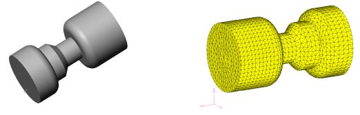
How can we put it all together? To simplify things at the beginning, let us assume that the solid is polyhedral (it has no curved surfaces). Note that we can still represent fairly complex shapes by approximating the surface with very small planar facets, as in the example below. A similar effect was achieved in the picture of the house in my CSG tree example earlier – where the cylinder was approximated by a series of facets.
Let us look at the bookkeeping we need to do for storing the 3D data of a solid. A simple boundary model will store data about faces, edges, and vertices. We could just list all the data of the solid face-by-face. But in doing so, we will repeat the information of each edge two times (since each edge is a part of two faces). Likewise, we need to store the three coordinates for each vertex - and each vertex is shared by several edges. So these coordinates will be repeated many times. A better scheme is shown below:
This data structure can be used for any polyhedral solid, even with a large number of faces. If can be used to write algorithms to answer any question about the solid that we have mentioned before (calculate volume, weight, center of mass, find if a given point is inside or outside, etc). But these algorithms tend to be inefficient. Say we need to calculate the surface area. We do so by adding the area of each face. Consider a face on a part as shown below.
It has two ‘holes’. A possible algorithm to compute the area of this face looks like:
Step 1. Separate all edges into three subsets,
E1 = edges of the outer 'loop', E2 = edges of the
triangle-shaped loop inside, and
E3 = edges of the rectangular loop inside.
Step 2. Compute the area of each loop, AE1, AE2, AE3.
Step 3. Area of Face = Area of outer loop - sum of area of all inner loops.
If we had originally stored the edges of each loop separately, we would save the effort of Step 1. In fact, several other algorithms we need to perform other useful tasks are inefficient using this scheme. A better scheme was proposed by Baumgart - it uses a larger storage space, but makes many algorithms easy to implement. It was called the winged-edge data structure. We look briefly at a simplified version of this structure. First, let us list a few operations that can be performed efficiently with the extended data structure:
To allow the above operations, we shall adopt some conventions which are useful: Note that each face has exactly one outer-loop of edges, and may have several holes, each of which makes an inner loop on the face. Our convention is that we shall list all edges on a loop as follows: For the outer loop, we will list the edges in sequence that allows us to go around the face in a counter clockwise direction, when looking directly at the face from outside. For each inner loop, we will list the edges in a way that we travel clockwise, when looking at the face.
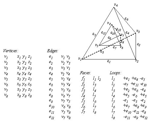
Observe that each edge on a solid is shared by exactly two faces. Each edge has a direction - from it's start vertex to its end vertex. If we were traveling along the positive direction of this edge when traveling on the loop containing it in one face, we must be traveling in its reverse direction when going around the loop on its neighboring face. This led to the idea of splitting each edge into two coincident edges (called co-edges) -- one in the positive direction, and the other in the reverse direction (look at edge e4 in the figure below). The geometry of the faces is then stored in terms of loops made up of co-edges, not edges. In some CAD systems, co-edges may be called half-edges. We are now ready to construct a simple example.
The figure below shows this data structure for a tetrahedron, with a smaller tetrahedron cut away from one face. This demonstrates the data stored for each object in our data structure. I am using the convention that the first loop for each face is the outer loop (counter clockwise), and all subsequent loops are inner loops (hence, clockwise). In the figure, the data is stored in terms of co-edges, which refer back to their base geometric entities - line segments. The co-edges are shown with + or - signs, according to their direction relative to the corresponding directed edge.
Within the computer, each entity, such as face, loop, co-edge, vertex and its data is stored in a structure (or class). A solid is a list of faces; a face is a list of loops; a loop is a list of co-edges; a co-edge points to its start-vertex and its end-vertex. The connections between these objects for a solid are maintained by a pointers. The figure below shows a typical data structure.